Visually exploring local explanations to understand complex machine learning models

Professor Di Cook
Monash University

@visnut@aus.social

Outline

• Example data: penguins
• Tours: visualising high-dimensions with linear projections
• XAI and local explanations
• Demo

Example data: Palmer penguins

See Allison Horst’s web site on the penguins data for more details.

Pre-process data

penguins <- penguins %>%
  na.omit() # 11 observations out of 344 removed
# use only vars of interest, and standardise
# them for easier interpretation
penguins_sub <- penguins[,c(1, 3:6)] %>% 
  mutate(across(where(is.numeric),  ~ scale(.)[,1])) %>%
  rename(bl = bill_length_mm,
         bd = bill_depth_mm,
         fl = flipper_length_mm,
         bm = body_mass_g)
summary(penguins_sub)

#>       species          bl              bd              fl       
#>  Adelie   :146   Min.   :-2.17   Min.   :-2.06   Min.   :-2.07  
#>  Chinstrap: 68   1st Qu.:-0.82   1st Qu.:-0.79   1st Qu.:-0.78  
#>  Gentoo   :119   Median : 0.09   Median : 0.07   Median :-0.28  
#>                  Mean   : 0.00   Mean   : 0.00   Mean   : 0.00  
#>                  3rd Qu.: 0.84   3rd Qu.: 0.78   3rd Qu.: 0.86  
#>                  Max.   : 2.85   Max.   : 2.20   Max.   : 2.14  
#>        bm       
#>  Min.   :-1.87  
#>  1st Qu.:-0.82  
#>  Median :-0.20  
#>  Mean   : 0.00  
#>  3rd Qu.: 0.71  
#>  Max.   : 2.60

Examine the penguins using a tour

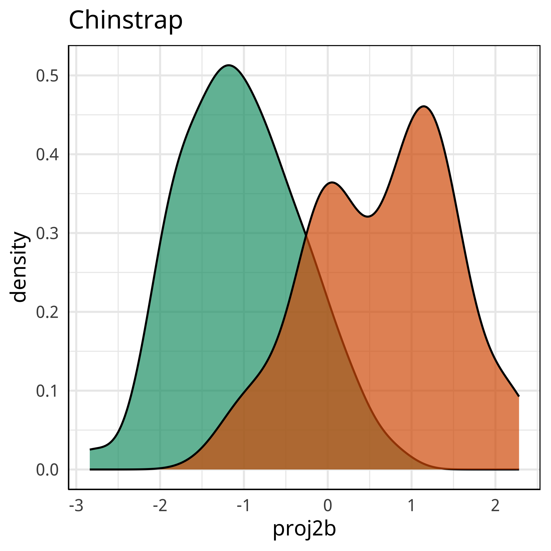
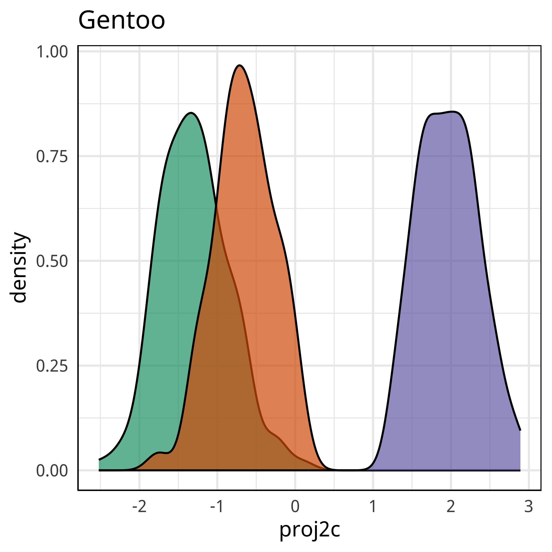
Grand tour: randomly selecting target planes

Adelie

Chinstrap

Gentoo

Examine the penguins using a tour

Grand tour: randomly selecting target planes

Guided tour: target planes chosen to best separate classes

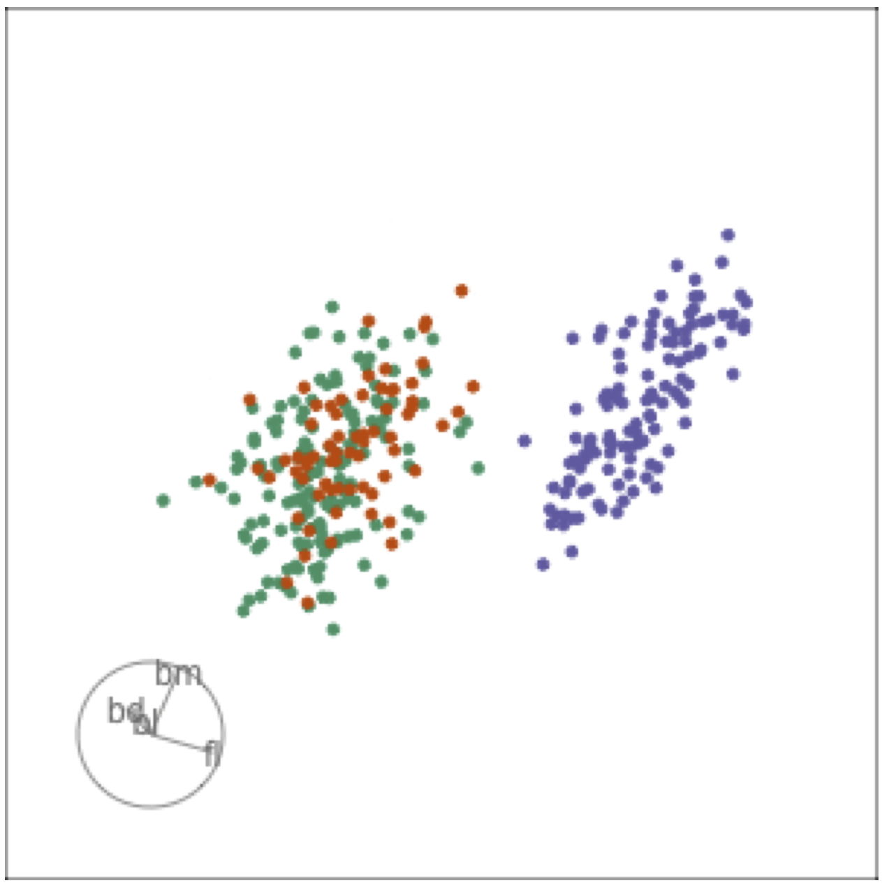
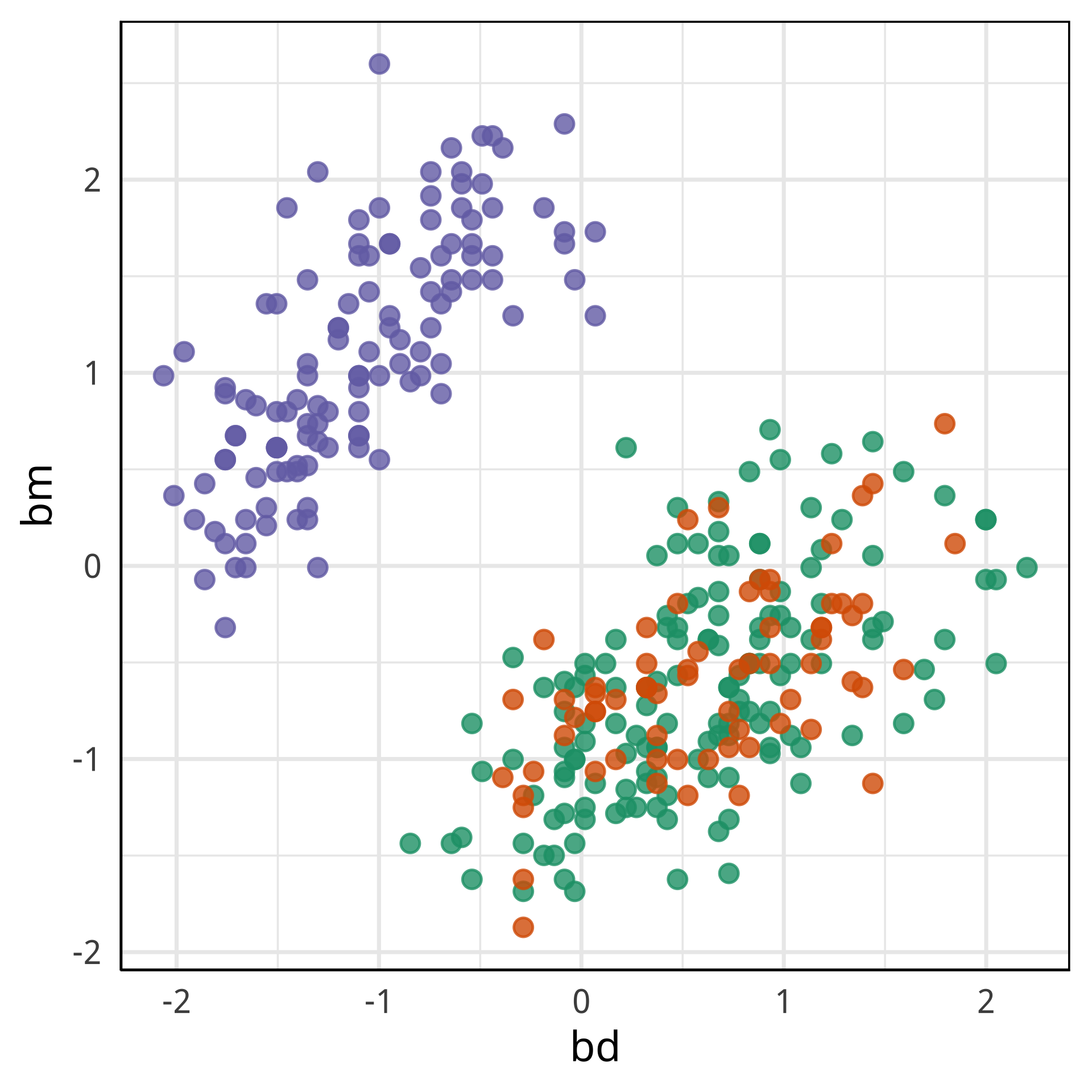
Tour projections are biplots

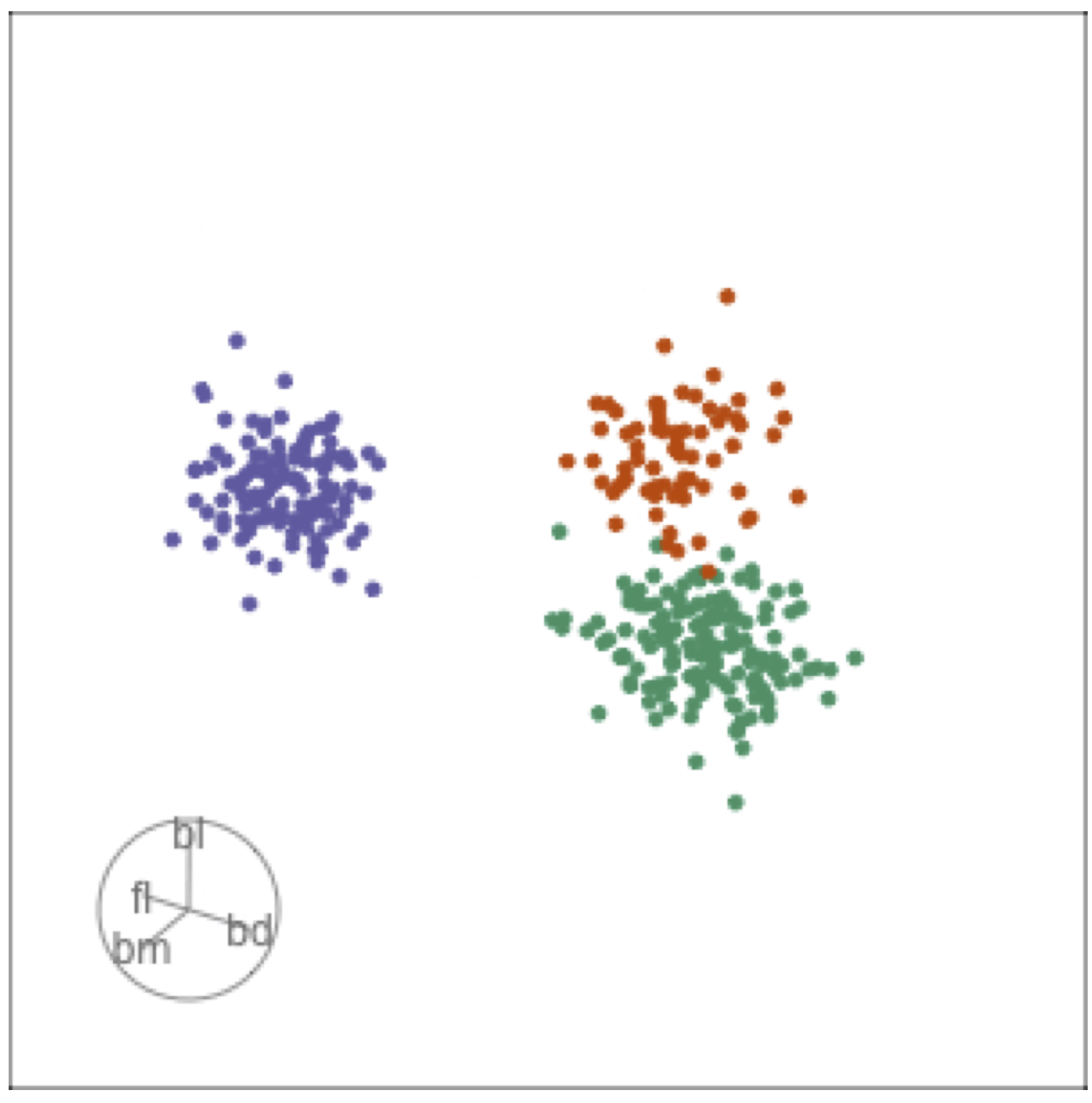
bd and bm distinguish Gentoo

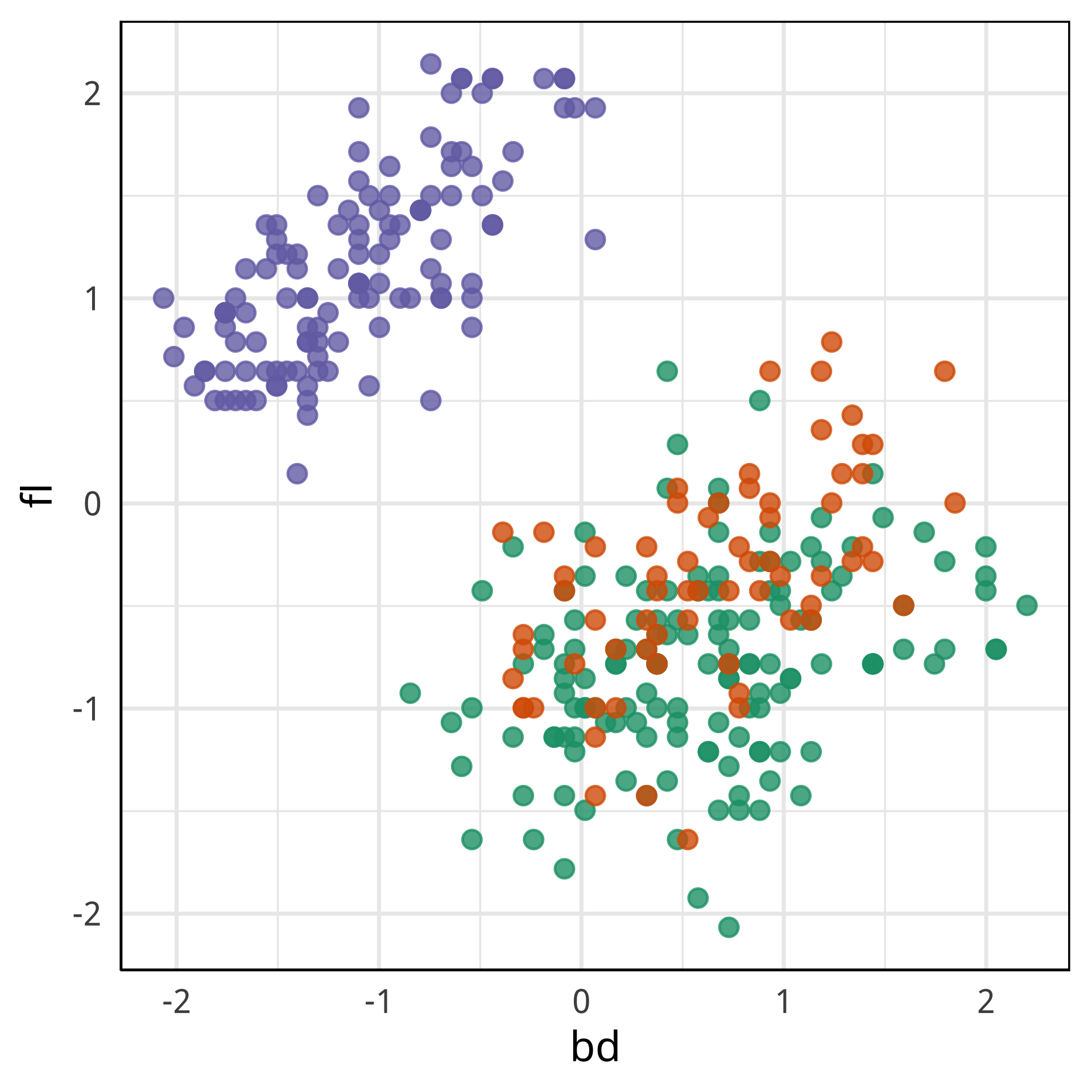
Tour projections are biplots

bd and fl also distinguish Gentoo

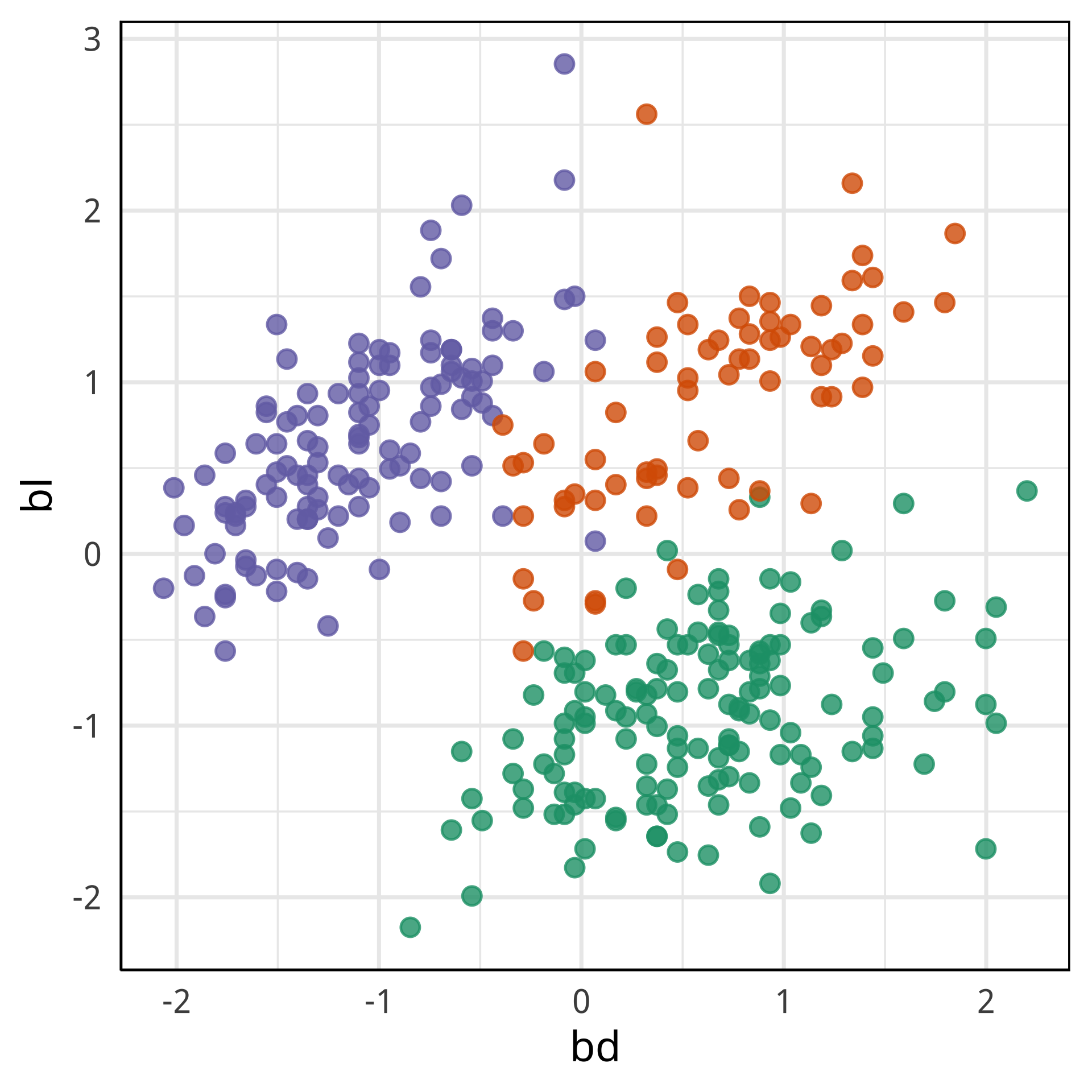
Tour projections are biplots

bd and bl distinguish Chinstrap from Adelie

Fit a classification model

library(randomForest)
set.seed(2311)
penguins_rf_cl <- randomForest(species~., penguins_sub, 
                            ntree = 1000,
                            importance = TRUE)

#> 
#> Call:
#>  randomForest(formula = species ~ ., data = penguins_sub, ntree = 1000,      importance = TRUE) 
#>                Type of random forest: classification
#>                      Number of trees: 1000
#> No. of variables tried at each split: 2
#> 
#>         OOB estimate of  error rate: 2.4%
#> Confusion matrix:
#>           Adelie Chinstrap Gentoo class.error
#> Adelie       143         3      0      0.0205
#> Chinstrap      4        64      0      0.0588
#> Gentoo         0         1    118      0.0084

Variable importance (globally)

#>    Adelie Chinstrap Gentoo MeanDecreaseAccuracy MeanDecreaseGini
#> bl  0.454      0.38  0.098                 0.31               88
#> bd  0.080      0.13  0.299                 0.17               40
#> fl  0.128      0.12  0.336                 0.20               67
#> bm  0.015      0.14  0.154                 0.09               18

Globally, bl, fl are most important, and to a lesser extent, bd and even lesser extent bm. (Note: one needs to play with sign.)

lin1 <- penguins_rf_cl$importance[,4]/
           sqrt(sum(penguins_rf_cl$importance[,4]^2))
# Flip sign of one
lin1[2] <- -lin1[2]
proj1 <- as.matrix(penguins_sub[,-1])%*%as.matrix(lin1)
penguins_pred <- penguins_sub %>% 
  mutate(proj1=proj1)

Variable importance (by class)

#>    Adelie Chinstrap Gentoo MeanDecreaseAccuracy MeanDecreaseGini
#> bl  0.454      0.38  0.098                 0.31               88
#> bd  0.080      0.13  0.299                 0.17               40
#> fl  0.128      0.12  0.336                 0.20               67
#> bm  0.015      0.14  0.154                 0.09               18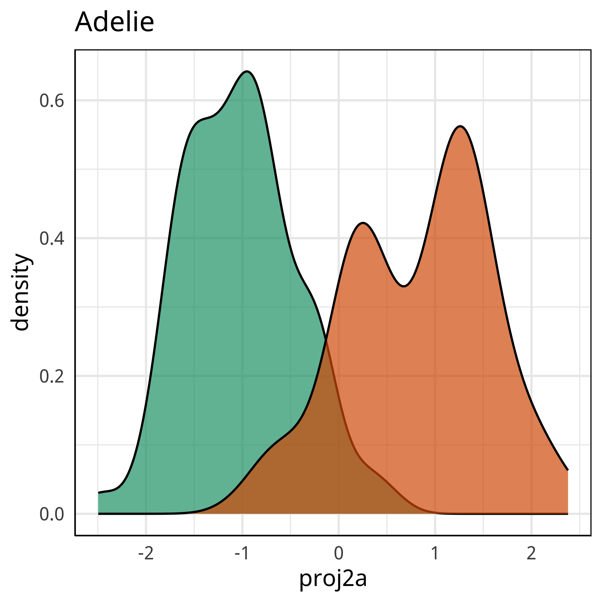

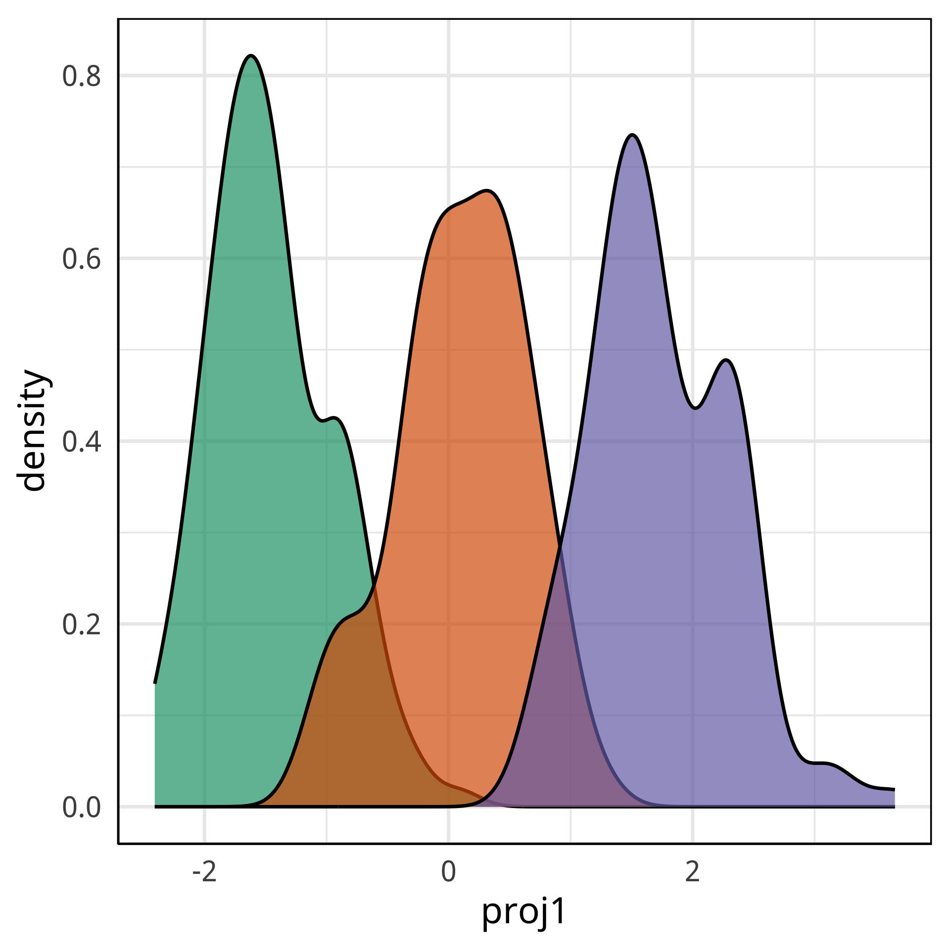
Note: one still needs to play with sign.

Radial tours: bd is very important

A radial tour changes the contribution for one variable, reducing it to 0, and then back to original.

At right, cofficient for bd is being changed.

When it is 0, gap between Gentoo and others is smaller, implying that bd is very important.

but bl is less important

At right, the small contribution for bl is reduced to zero, which does not change the gap between Gentoo and others.

Thus bl can be removed from the projection, to make a simpler but equally effective combination of variables.

View of the model

set.seed(1124)
penguins_grid <- tibble(bl=runif(1000, -3, 3),
                       bd=runif(1000, -3, 3),
                       fl=runif(1000, -3, 3),
                       bm=runif(1000, -3, 3))
penguins_grid <- penguins_grid %>%
  mutate(pred = predict(penguins_rf_cl, penguins_grid))
load("data/penguins_pp.rda")
proj <- as.matrix(pp$basis[[dim(pp)[1]]])
penguins_grid <- penguins_grid %>%
  mutate(pp1 = as.matrix(penguins_grid[,1:4])%*%proj[,1],
         pp2 = as.matrix(penguins_grid[,1:4])%*%proj[,2])

Global importance cannot provide a single linear view revealing all aspects of the model.

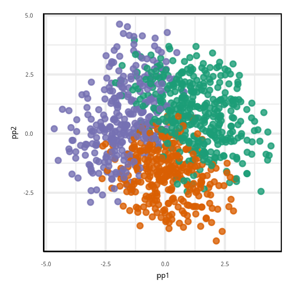
Local explanations

Explainable Artificial Intelligence (XAI) is an emerging field of research that provides methods for the interpreting of black box models¹.

A common approach is to use local explanations, which attempt to approximate linear variable importance in the neighbourhood each observation.

Fitted model may be highly nonlinear. Overall linear projection will not accurately represent the fit in all subspaces.

1. Adadi and Berrada 2018; Arrieta et al. 2020

Compute SHAP values

Each observation has a variable importance, computed using the SHAP method.

Common methods for local explanations

• SHAP is computed at each observation, by examining predictions while varying one variable and holding others fixed at mean, see Molnar (2022) Interpretable Machine Learning.
• LIME examines predictions at each observation from randomly generated new observations in local neighbourhood, see Mason (2020).

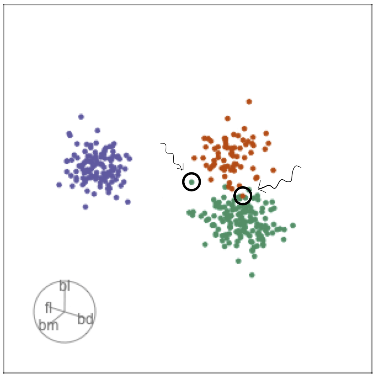
Comparing local explanations of all

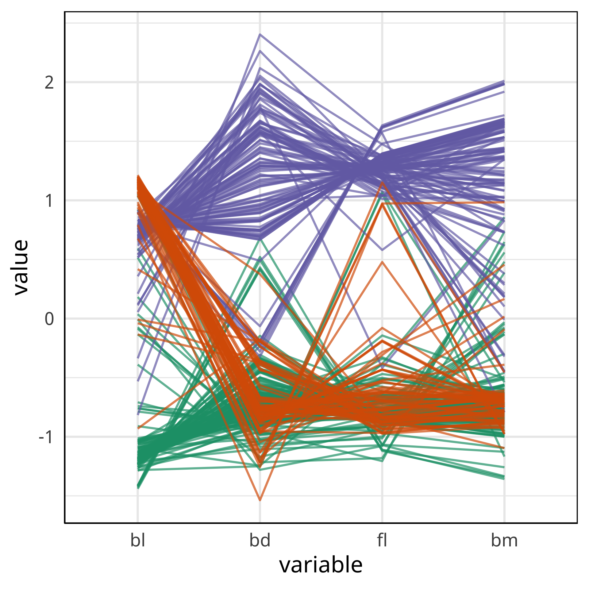
Observations with different local explanations from the rest of their group are likely the misclassified cases.

And from the parallel coordinate plot can be seen which variables are most contributing to this.

Demo

Exploring the local explanations, with a radial tour, using cheem: https://ebsmonash.shinyapps.io/cheem_initial/

What we learn

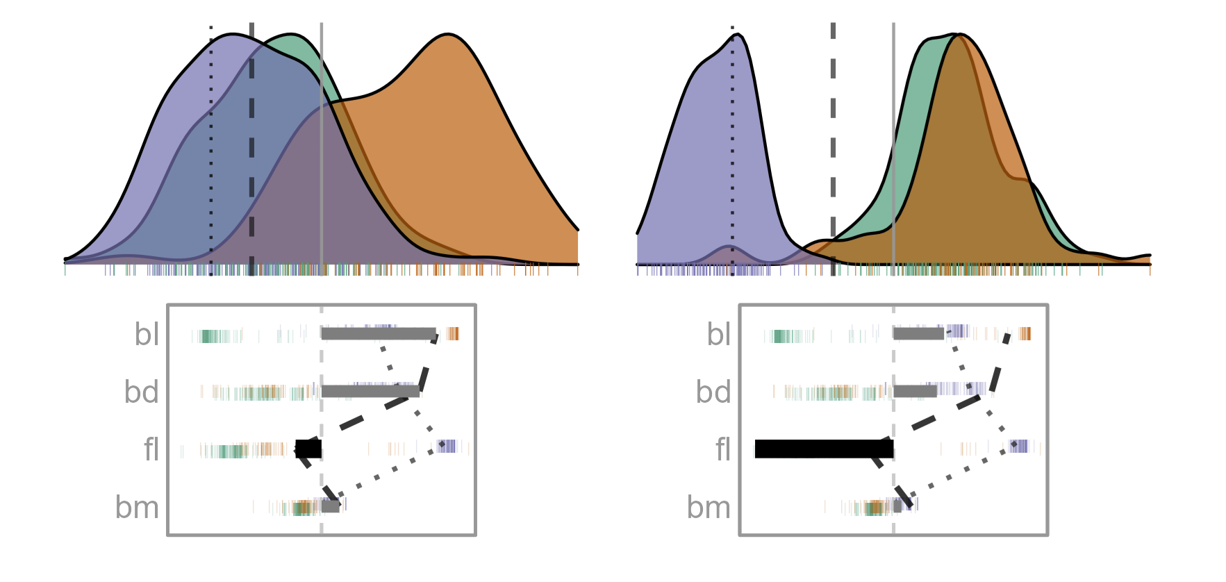
For this Gentoo penguin, mistaken to be a Chinstrap, the model used only a small component of fl, unlike the other Gentoo but more like the bulk of the Chinstrap penguins. The fl component is an important difference between this penguin and others in it’s species.

What we learn

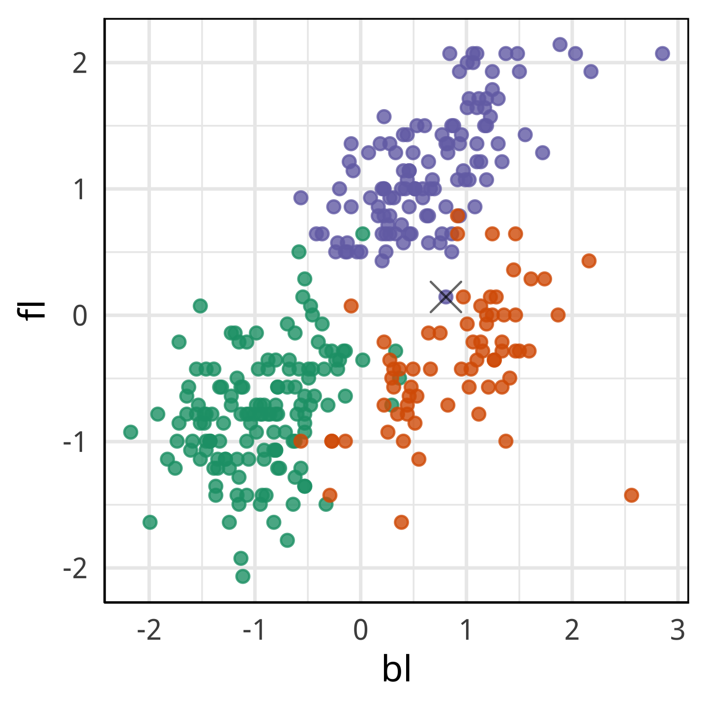
With fl it looks more like a Chinstrap.

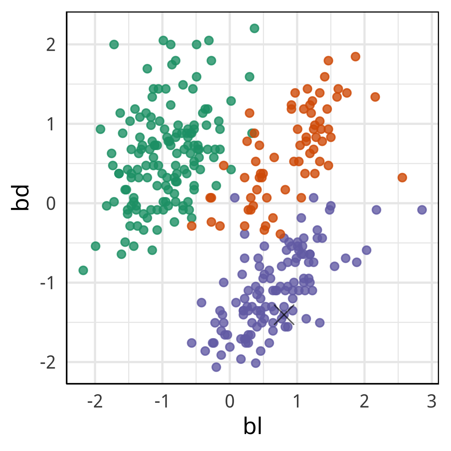
With only bl and bd it looks like it’s own species.

Summary

• Local explanations tell us how a prediction is constructed, for any observation.
• User-controlled, interactive radial tours are useful to check the local explanations, and better understand a model fit in local neighbourhoods.

Further reading

This work is based on Nick Spyrison’s PhD research, developed after discussions with Przemyslaw Biecek.

• Spyrison, Cook, Biecek (2022) Exploring Local Explanations of Nonlinear Models Using Animated Linear Projections
• R package: cheem and shiny app for experimenting.
• Wickham, Cook, Hofmann (2015) Visualizing statistical models: Removing the blindfold.

Acknowledgements

Slides produced using quarto.

Slides available from https://github.com/dicook/Stellenbosch_2022.

Viewable at https://dicook.github.io/Stellenbosch_2022/slides.html.